Introduction: Taming an Unstable Bottleneck
Imagine trying to compress information in a machine learning model by turning a "compression knob," only to find nothing happens until BANG! suddenly your model drastically changes behavior. This is the classic challenge in the Information Bottleneck (IB) framework. The IB trade-off involves squeezing a source X into a compressed representation Z while preserving as much information as possible about a target Y. By tuning a parameter (often called β), we decide how much we care about compression vs. prediction.
Standard IB solutions often behave like a stubborn valve: nothing comes out until a critical pressure is reached, and then it erupts all at once. These abrupt leaps, known as phase transitions, make it difficult to have fine-grained control over model compression.
In theory, as we increase β gradually, we'd expect the representation to slowly lose less-important details. In practice, standard IB solutions often behave like a stubborn valve: nothing comes out until a critical pressure is reached, and then it erupts all at once. These abrupt leaps known as phase transitions mean the optimal encoding p(z|x) can change suddenly at certain β values (analogous to water instantly freezing into ice when it gets cold enough). Such instability is more than a quirk; it's a serious obstacle if we want fine control over model compression or need smooth adaptation.
Faruk Alpay (ORCID: 0009–0009–2207–6528) tackles this problem head-on in his project "Stable and Convexified Information Bottleneck Optimization via Symbolic Continuation and Entropy-Regularized Trajectories." The goal is simple to state but hard to achieve: make the IB optimization stable and gradual, so that increasing the β "knob" leads to a smooth evolution of the representation without sudden jumps. In this article, we'll unpack the key ideas behind this new IB solver, see how it behaves on example problems, and understand what makes it unique in practice.
The Information Bottleneck Problem (and Its Quirks)
The IB framework is a powerful tool for representation learning. It defines an objective that balances compression (measured by how much information Z retains about X, denoted I(Z;X)) against prediction quality (how much information Z has about target Y, denoted I(Z;Y)). By adjusting β, one navigates between a highly compressed but less informative Z (high I(Z;X) penalty) and a more detailed Z that captures Y well (low penalty on I(Z;X)).
In practical terms, IB can help distill datasets, reduce overfitting, or even interpret neural networks by finding a bottleneck representation that doesn't throw away the task-relevant bits.
The Information Bottleneck method provides a principled approach to extracting relevant information from complex data. It's not just about compression—it's about finding the minimal sufficient statistics that preserve what matters.
However, a notorious phenomenon occurs when you sweep β through different values: phase transitions. At certain "critical" β thresholds, the optimal Z abruptly changes structure. For instance, below a threshold the best strategy might be to lump several inputs together (losing some detail because compression is cheap), but just above that threshold, it suddenly becomes worthwhile to split those inputs into separate clusters to gain more predictive power.
The result is a discontinuity: key metrics like I(Z;Y) can jump suddenly, and the encoder p(z|x) can reconfigure overnight. These transitions were extensively studied in IB theory; they're mathematically akin to phase changes in physics. While intellectually intriguing (the system "discovers" a new cluster or feature at a precise point), they pose a problem for anyone who wants incremental control.
If you're tuning β slowly, an unexpected jump can break the smooth flow of training or make model behavior unpredictable in sensitive applications. Ideally, we want an IB solver that evolves gradually, so that each small increase in β yields a small, understandable change in the representation.
A New Approach: Convexify and Continue
To eliminate these abrupt jumps, Alpay's method introduces two clever modifications to the IB objective, followed by a novel solving strategy:
1. A Convex Compression Penalty
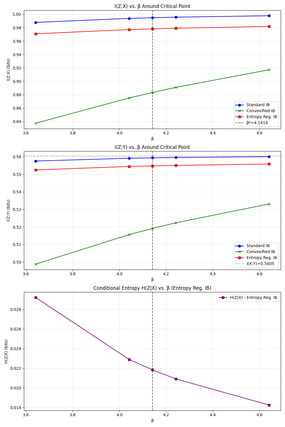
Instead of penalizing I(Z;X) linearly with β (which leads to a non-convex optimization and a rugged landscape), the method uses a strictly convex function of I(Z;X), for example u(I(Z;X)) = [I(Z;X)]². Intuitively, this "convexified" penalty smooths out the optimization landscape. Small changes in I(Z;X) now have a gradually increasing cost, which discourages the solution from staying stuck in a plateau and then leaping off a cliff.
It's like rounding off sharp edges in the objective so the optimizer doesn't fall into a gap. The trade-off curve becomes gentler by construction, making it less prone to multiple optima fighting each other as β changes.
2. Entropy Regularization
In addition to the convex penalty, a tiny entropy term −εH(Z|X) is added to the objective. This term (with ε being small) encourages the encoder p(z|x) to retain a bit of randomness instead of making purely hard assignments. Why introduce randomness? Because hard deterministic cluster assignments are what cause those "spikes" and sudden jumps.
By keeping the encoder slightly probabilistic, the solution can morph gradually — probabilities can slowly shift from 90% to 99% instead of a flip from 0 to 1. This entropy regularization acts like a lubricant for the phase transitions.
3. Continuation via Predictor-Corrector
Perhaps the most innovative piece is how the solution is actually traced. Rather than solving the IB optimization from scratch for each new β (which would risk hopping to a new solution branch unpredictably), the method uses a continuation strategy. It treats β as a trajectory to move along, starting from a low β and incrementing it in small steps.
At each step, the algorithm predicts how the optimal encoder p(z|x) should change (using an analytically derived guide, essentially an ODE that tells us the direction of change), then corrects it by fine-tuning (ensuring it really is the optimum for the new β). This predictor-corrector method is akin to walking a tightrope with a pole: you anticipate the next lean and adjust continuously, rather than jumping to a whole new position.
The result is that the solver follows a single continuous branch of solutions without ever bifurcating to a different, discontinuous branch. If a standard IB solution would have split into a new cluster at β = 3, the continuation method instead witnesses that cluster emerging gradually. There's no mystery jump because we never let the solution wander away — each β's solution is tethered to the previous one.
By combining these ideas, the project delivers a solver that by design avoids sudden representation shifts. In essence, it turns the IB knob into a smooth dial. The approach draws on tools from information theory and convex optimization, but also from dynamical systems: treating the IB equations like a system to be gently steered through a potential rough patch.
It even monitors indicators of instability (like the curvature of the objective) along the way; if a phase transition is looming, the solver senses it (for example, a certain Hessian eigenvalue tends to zero) and takes appropriately small steps, eased by the entropy "lubricant," to glide through the would-be jump.
Smooth IB in Action: Binary Channel and Beyond
What does all this achieve in practice? To make it concrete, let's look at the two demo scenarios from the project's experiments: a Binary Symmetric Channel (BSC) and a structured 8×8 distribution. These are synthetic datasets chosen for their clear-cut phase transition behavior, perfect for before-and-after comparisons.
Binary Symmetric Channel (2×2 case)
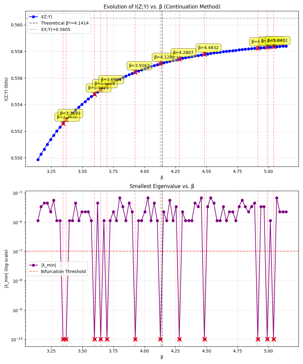
Here, X and Y are just binary bits with a noisy relationship (imagine Y is a flipped version of X with some probability). In the standard IB solution for this simple case, nothing much happens until β reaches a critical value around ~1.6. Below that, the optimal representation basically transmits no information about X (because the cost of even a bit of information is too high relative to the β penalty).
Then, at β ≈ 1.6, suddenly the optimal Z flips from "off" to "on," jumping to a state where it transmits a significant chunk of information about Y. If you plotted I(Z;Y) (how much info the bottleneck retains about Y) as a function of β, you'd see a flat line that suddenly shoots upward at that point. It's a quintessential phase transition.
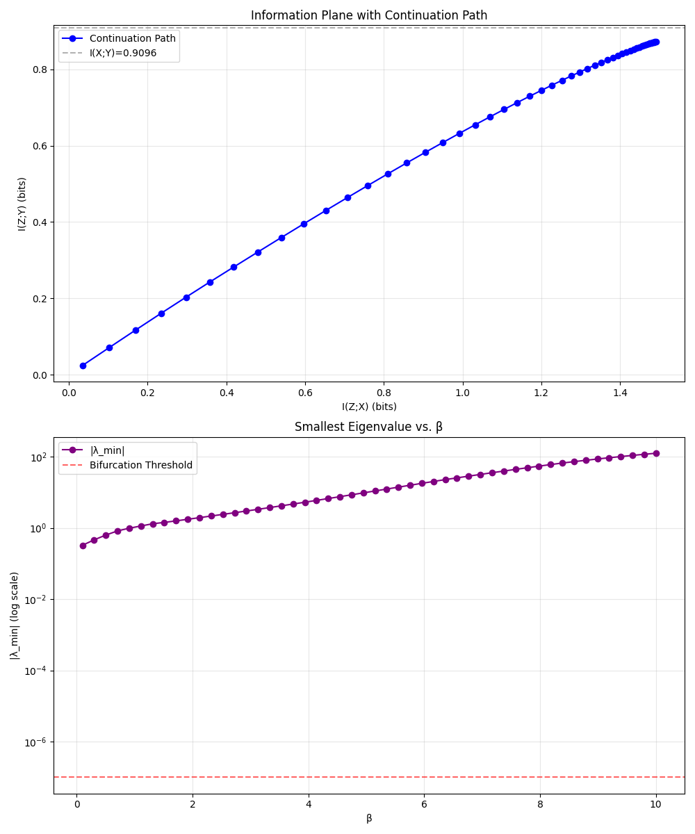
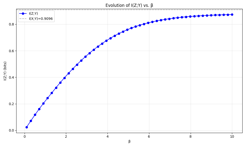
Now, with the convexified + entropy-regularized continuation solver, the same scenario plays out very differently. As β increases from 0, the solver starts to gently increase I(Z;Y) right away. There is no critical cliff at 1.6 — instead, the curve of I(Z;Y) rises gradually. By the time we pass β = 1.6, there's no drama; I(Z;Y) might accelerate a bit around that region, but smoothly, not abruptly.
Eventually, as β becomes large, the new method's I(Z;Y) converges to the same value as the standard IB (in this example, about 0.53 bits, which is the maximum mutual information between X and Y in this channel). In other words, both methods end up learning essentially the same optimal encoding in the limit, but the path taken is totally different. One is a step function; the other is a gentle curve.
The proposed solver achieves a stable trade-off curve where we can inspect any intermediate β and know the model didn't skip over a potentially useful gradual step.
To really hammer home that the phase transition is gone, Alpay also used a known diagnostic: tracking the smallest eigenvalue of the Hessian (a measure of curvature of the IB objective). In the standard IB, as β nears 1.6, this eigenvalue plummets to zero — a telltale sign of a bifurcation (much like how water's free energy curvature goes to zero at the boiling point).
In the new solver's trajectory, no such drop occurs; the curvature stays positive, meaning the solution branch remains stable and unbroken.
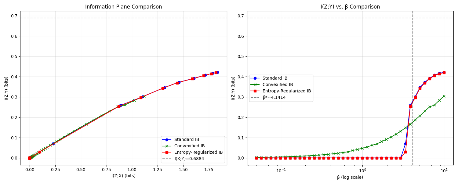
For readers not into the math details, the takeaway is that all indicators confirm a smooth ride: no hidden instability is lurking under the hood of the new method in the BSC example.
Hierarchical 8×8 Distribution
The second demonstration is more complex. Here we have 8 distinct input classes, and correspondingly, 8 possible outputs, arranged in a hierarchy. Think of it like 8 species of animals that are grouped into families: some share similarities in their Y distributions.
As β increases, an optimal IB encoder might first distinguish between broad families (say, splits the 8 into 2 big clusters), then later distinguish within those clusters (splitting into 3 or 4 clusters), and so on, until at very high β it might separate all 8 classes. Each time a new split becomes worthwhile, a phase transition would occur in the standard IB solution. So this scenario potentially has multiple phase transitions as we dial β from 0 upward — a perfect stress test for the solver.
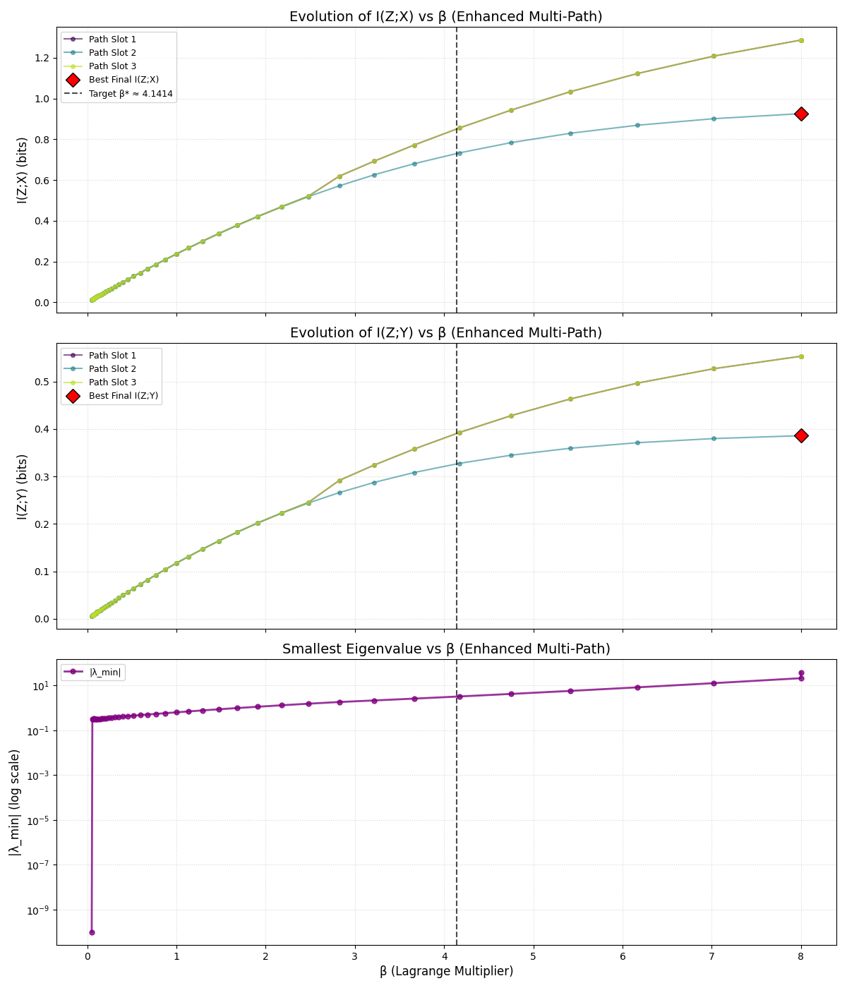
With the classic IB approach, you'd expect several sudden jumps in the encoding. By contrast, the convexified continuation method handles this scenario with grace. As β increases, clusters emerge one by one, but gradually.
With the classic IB approach, you'd expect several sudden jumps in the encoding. Indeed, if one were to run the standard IB algorithm here, you would see discrete jumps in the mutual information curves and abrupt changes in the encoding matrix p(z|x) at certain β thresholds (somewhere around β ~3 in one case, etc., corresponding to new clusters "popping" into existence).
By contrast, the convexified continuation method handles this scenario with grace. As β increases, clusters emerge one by one, but gradually. For example, rather than an instant split from 1 cluster to 2 at some magic β, you'd see the encoder probabilities slowly drifting until effectively two distinct clusters form. Then later, a third cluster forms in a similarly smooth fashion, and so on.
The transitions are so gentle that if you blink, you won't miss them — because there isn't a single blink-and-you-miss-it moment; the change spans a range of β values.
One way to visualize this is to look at the encoder p(z|x) itself as a heatmap over β. In the paper, the author shows snapshots of the encoding matrix at various β levels. Initially (very low β) the matrix is "fuzzy" — every x is mapped to z in a diffuse way (lots of mixed probabilities), reflecting heavy entropy regularization and little pressure to be accurate.
As β increases a bit, you start seeing structure: maybe two distinct columns emerge (meaning the encoder has effectively created 2 clusters of X). Increase β more, a third column brightens — now 3 clusters — and so forth until eventually 8 distinct columns are mostly lit (each input gets its own cluster at very high β).
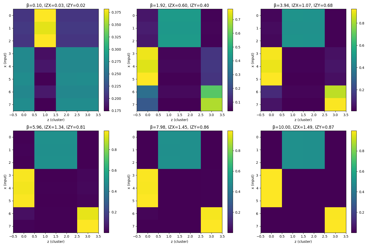
Importantly, none of these steps involve a harsh jump; it's a continuous morphing. In comparison, a standard IB encoder might have stayed completely fuzzy and then suddenly snapped into a 2-cluster state (with nearly binary 0/1 assignments) at a threshold, then hold until another snap to 4 clusters, etc. The new method's encoder is visually smoother when you compare them side by side.
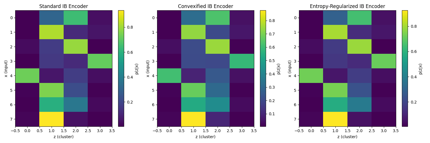
In a side-by-side snapshot at a fixed intermediate β, the standard IB encoder might look like crisp, high-contrast vertical stripes (hard clustering), whereas the convexified one will have more graded colors (soft assignments) — indicating that it hasn't made a harsh decision, which gives it the flexibility to adapt gradually.
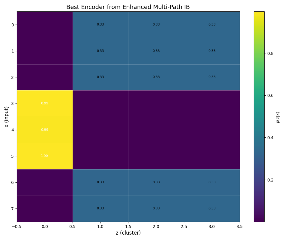
Crucially, this smooth ride doesn't come at the cost of final performance. By the time β is very large (meaning we care almost only about prediction, not compression), the new solver converges to essentially the same solution as standard IB: it recovers all 8 clusters and preserves basically all the mutual information I(Z;Y) that is possible (which in this constructed example approaches the entropy of Y).
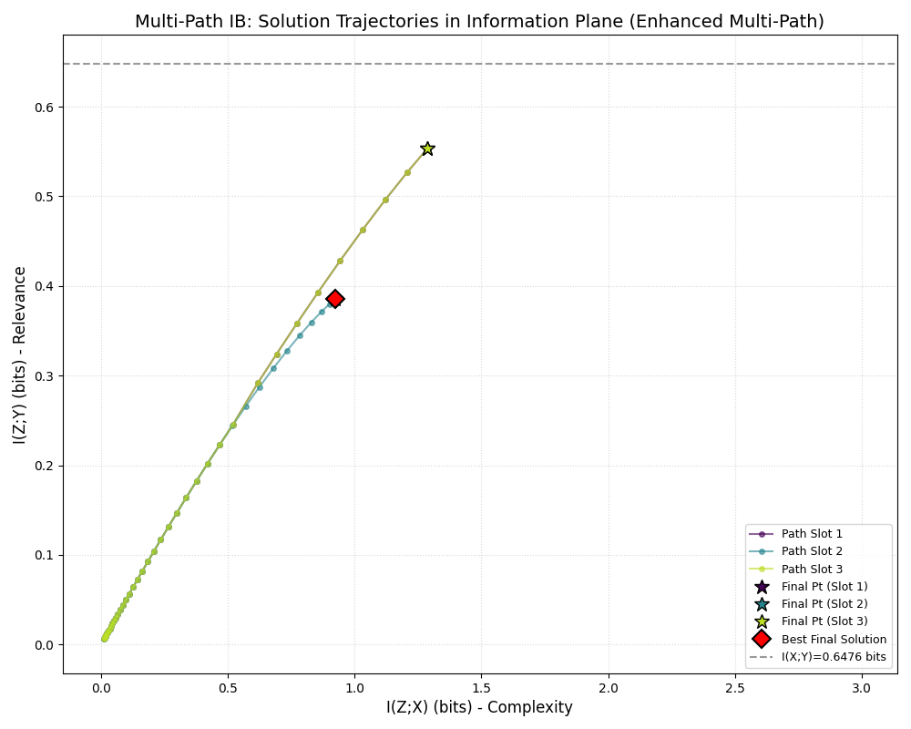
In the intermediate β regimes, something interesting happens: because the method avoids rash jumps, it actually explores representations that standard IB might miss. For example, at a medium β, standard IB might stubbornly stick to, say, 2 clusters until it can jump to 4, whereas the new method might already be smoothly transitioning through 3 clusters.
During that transition, it could achieve a higher I(Z;Y) than standard IB at the same compression level, simply because it allowed a third cluster to exist partway. In essence, the convexified approach can yield better trade-offs at certain points because it doesn't "hesitate" or overshoot. All the while, it maintains stability — there's no wild oscillation or random trial-and-error; everything follows one continuous path.

Why Does This Matter? (Practical Usability)
You might wonder, beyond these toy examples, what is the practical significance of having a stable IB solver. For researchers and engineers, there are a few clear advantages:
Smooth Exploration of Trade-offs
If you want to study how compression affects your model's knowledge, the continuation approach gives a complete, smooth trajectory of solutions. No more guessing where the phase transitions are — you can literally see the representation evolve and pick a β that gives you just the right balance. This is especially useful in model compression or pruning scenarios, where you might want to gradually simplify a model and monitor performance.
Reliability in Sensitive Settings
In scenarios like continual learning or real-time systems, you might need to adjust the "compression knob" on the fly. An unstable IB could cause a sudden drop or surge in performance at the wrong time. The stable IB framework promises reliable gradual adaptation — crucial for deployment in dynamic environments.
Imagine a communication system that adapts its compression level based on bandwidth: you wouldn't want it to suddenly throw away important information or overload the channel because of a phase transition. The convexified IB would adjust smoothly.
Single Run, No Tuning Gymnastics
Previously, one way to cope with IB's jumps was to run many random initializations or "multi-path" solvers. Essentially, you'd try to find alternate solutions around the jump or run a new optimization after the jump and hope you catch the better one.
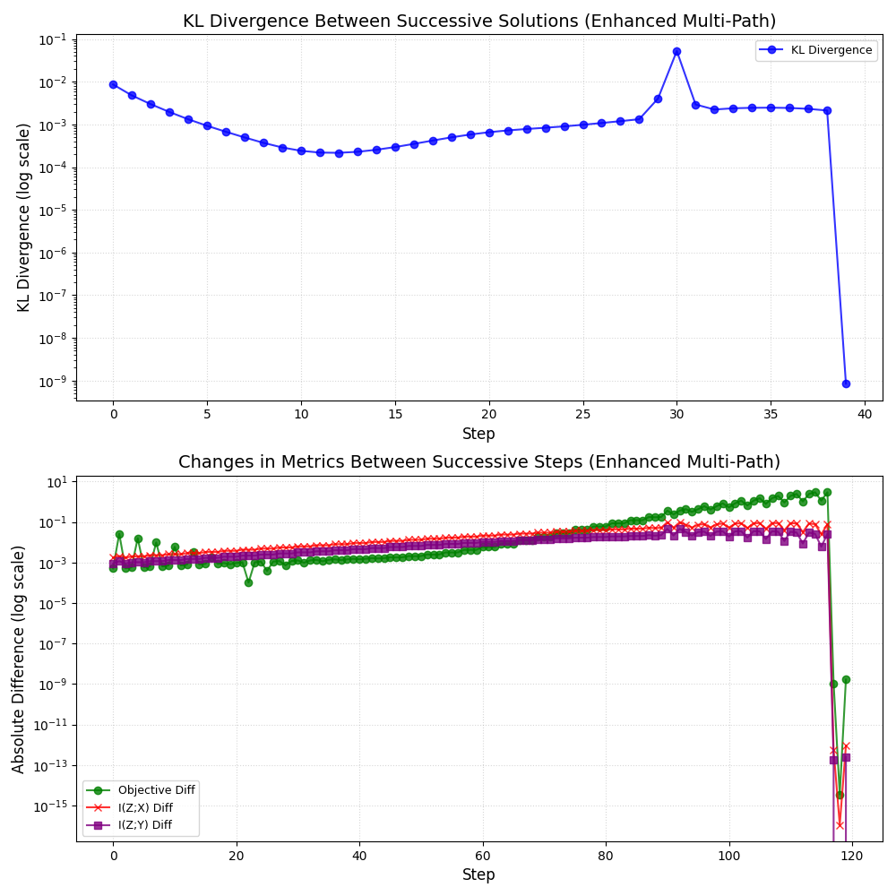
Alpay's solver eliminates that hassle. With the predictor-corrector continuation, one run suffices to track the optimal path. This not only saves computation, it ensures you don't accidentally miss a better solution or fall off on a suboptimal branch. The code implements step-size control and monitors stability metrics automatically, so it's robust out-of-the-box.
General Insight and Extensibility
Convexifying the objective and adding entropy regularization could be beneficial ideas beyond these examples. It hints that other information-theoretic objectives (or even training neural nets with information bottleneck-inspired losses) might benefit from a similar treatment to avoid instability.
In that sense, this project opens a door: it paves the way for using IB principles in scenarios that were previously daunting due to those phase transitions. Now that we can tame the IB, we might integrate it into deep learning training routines or use it for interpretability research with more confidence.
Conclusion: A Smoother Road Ahead for IB
In summary, "Stable and Convexified IB Optimization via Symbolic Continuation" delivers exactly what its name promises: a stable, convexified approach to the information bottleneck problem that turns unpredictable leaps into smooth trajectories. By blending convex optimization tricks with a continuation (homotopy) method and just a dash of randomness for smoothness, Faruk Alpay's solver charts a continuous path through the IB landscape.
The Information Bottleneck has always been a powerful theoretical framework, but its practical applications were limited by phase transitions. This work bridges the gap between theory and practice by making IB more stable and predictable.
It demonstrates its power on both simple and complex synthetic tasks, eliminating abrupt phase transitions while matching the performance of standard IB in the end. The solver is not just a theoretical exercise; it's a practical tool. Anyone working with information bottleneck ideas can try it out and benefit from the improved stability and clarity it provides.
The project's code (with an easy-to-run demo) and the detailed paper are openly available. The repository even includes all the figures we discussed, generated by the demo script, so you can reproduce and visualize the results yourself. Feel free to explore the paper and code on GitHub to dive deeper into the math or to apply this solver to your own data. The hope is that this work will enable wider adoption of IB methods in real-world ML systems, where gradual and reliable behavior is a must.

Ready to experiment or learn more? You can find the full paper and the open-source code in the GitHub repository. Check it out here: Stable Continuation IB on GitHub.
